Introduction
ETA squared is a measure of effect size that Stata can easily estimate after regression or ANOVA procedures. In this blog, we’ll show you how to use Stata to calculate ETA squared for entire models and individual predictor variables.
Load Data
Let’s load Stata’s automobile dataset:
sysuse auto
describe
ETA Squared after Regression
Try the following code:
regress mpg weight i.foreign

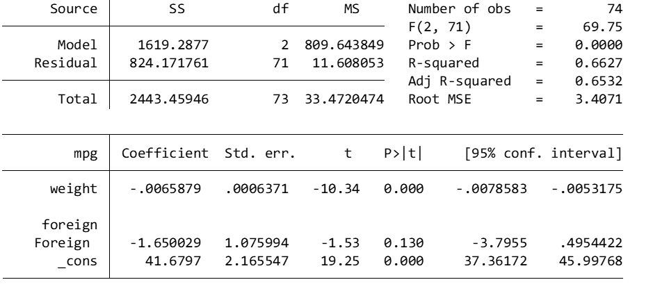
Adjusted R squared tells you that the regression explains 65.32% of the variation in mpg, but there aren’t separate effect sizes for the predictors of weight and foreign origin. Now try:
estat esize

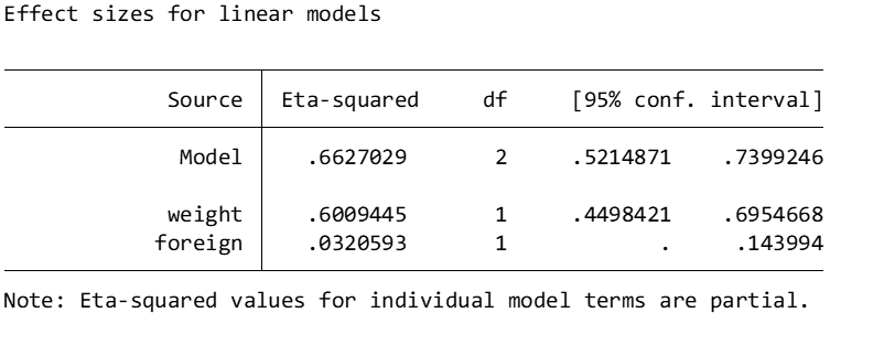
Helpfully, we learn that over 60% of the variation in mpg is explained by the weight of the car; the foreign origin of the car is much less explanatorily powerful. One of the advantages of the ETA squared postestimation command is the availability of ETA squared for each predictor.
ETA Squared after ANOVA
Let’s try an ETA squared postestimation after an ANOVA conducted on another dataset:
sysuse voter
anova pop candidat inc
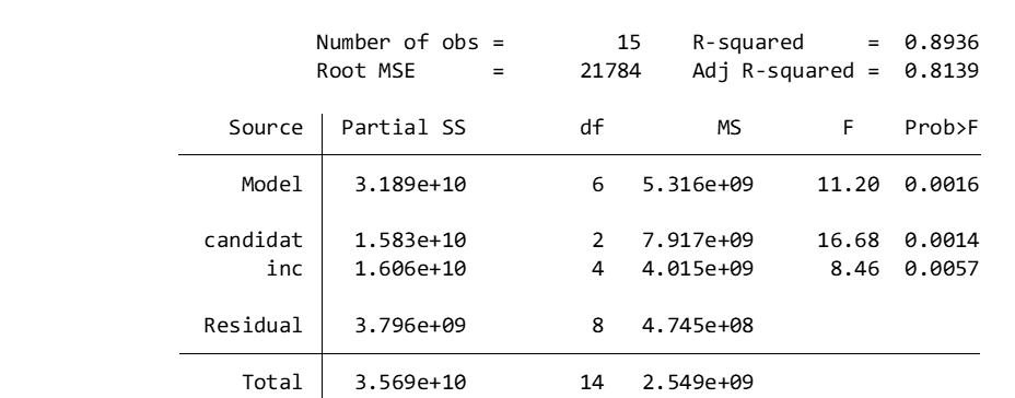
Here, we are trying to model population as a function of an area’s preferred candidate and income level:

Next, enter:
estat esize
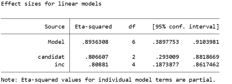
And you get back:

So the variation in population is roughly equally explained by candidate selection and income.
BridgeText can help you with all of your statistical analysis needs.


