Introduction
Log transformations can be used for many purposes in statistical analysis. In this blog entry, we’ll explain one scenario in which a log transformation is particularly useful in demonstrating a trend. Fortunately, log transformations are easy to achieve in Stata.
Create Data
First, we’ll create mock data, then we’ll show you how to carry out a log transformation.
set obs 30
gen subj = _n
label variable subj "Subject #"
gen q1_a = runiform(1,7)
gen q2_a = runiform(1,7)
gen q3_a = runiform(1,7)
gen q4_a = runiform(1,7)
gen q1 = round(q1_a)
gen q2 = round(q2_a)
gen q3 = round(q3_a)
gen q4 = round(q4_a)
drop q1_a q2_a q3_a q4_a
gen y = q1 * q2 * q3 * q4
egen x = rowmean(q1 q2 q3 q4)
sort y
replace y = 70000 in 30
Visualize Data
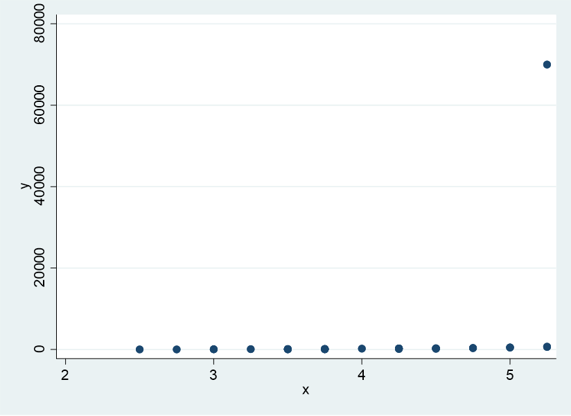
Let’s assume that we’re going to regress y on x. Begin with a scatterplot:
scatter y x

There’s no trend visible. However, when we run the regression, it’s significant at p < .10.
regress y x

The scatter plot and visual inspection of the data reveal the existence of a massive outlying data point at which y = 70,000. All of these conditions suggest the possible usefulness of log-transforming y.
Log Transformation
Let’s create a log-transformed version of y using:
gen lny = ln(y)
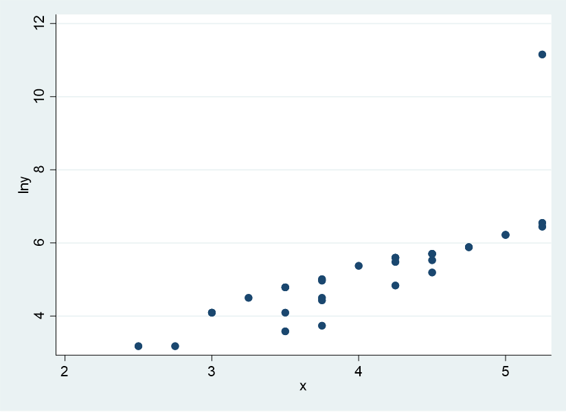
And now let’s create a scatter plot again, this time with the log-transformed y.
scatter lny x

A trend is now clear, and, if you run the regression again, it becomes significant at p < .0001.
regress lny x

Log-transformation was therefore particularly useful in reducing the inordinate influence of the single outlying data point of y = 70,000 and revealing the underlying trend.
BridgeText can help you with all of your statistical analysis needs.


