One of the most basic questions that comes up in quantitative research projects is whether the mean of one variable is different from the mean of another variable. Are men taller than women? Do people with degrees earn more than people without degrees? Do blondes get more dates than brunettes? These are all questions whose answer depends on comparing a mean between two groups. Today, we’ll discuss how to conduct quantitative research of this kind by means of a independent samples t-test in which variances between groups are unequal.
Remember, before you can conduct an independent samples t-test, you need the following to be true.
- The cases need to be independent. There can be no overlap between the two groups that are being compared.
- The dependent variable needs to be at the continuous level of measurement.
- The variances of the two groups need to be similar.
- The dependent variable needs to be approximately normal.
First, let’s generate some data on gender and height using Stata.
set obs 40
gen subj = _n
label variable subj "Subject #"
gen gender = .
replace gender = 1 in 1/20
replace gender = 2 in 21/40
label define gender 1 "Women " 2 "Men"
label variable gender "Gender"
label value gender gender
drawnorm height1, mean(153) sd(10)
drawnorm height2, mean(185) sd(27)
replace height1 = . in 21/40
replace height2 = . in 1/20
egen height = rowmax(height1 height2)
drop height1 height2
label variable height "Height"
We can already tell that the cases are independent, because each subject is either a man or a woman. We know that the dependent variable, height, is a continuous variable with a mean of 164.17 centimeters (SD = 24.63).

Next, we can use the sdtest command in Stata to compare variances in height between the two classes.

Here, we reject the null assumption that variances are equal, because Ha: ratio ≠ 1 has a p value less than .05 (specifically, p = .002). Next, we’ll test the normality of the distribution of the dependent variable of height using the Shapiro-Wilk test. If the p value of a Shapiro-Wilk test is < .05, then the assumption of normality is upheld. Below, we see that height is distributed normally for men and women (check the Prob>z) column for p values.

Because our assumption of equal variances was violated, we need to run an independent samples t-test based on an assumption of unequal variances.

Here we see that mean female height (M = 150.98, SD = 12.66) is significantly less than mean male height (M = 177.36, SD = 26.81), t(27.08) = -3.98, p = .0002. We’re done!
Of course, you could go a step further by calculating the effect size (with an unequal variances assumption built in) of the difference and reporting the statistical power of your findings.

The effect size of the difference, d = -1.26, is interpreted as a very large difference. How about the achieved statistical power?

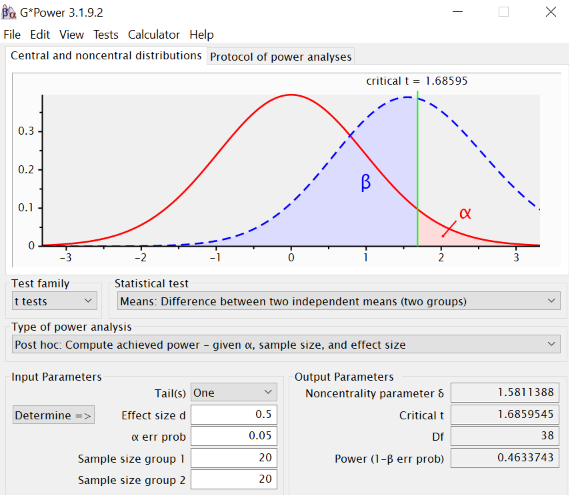
The power—assuming our one-sample hypothesis setup (men are taller than women), selection of p = .05, detectable effect size of 0.5, and 20 people in each group—is only 0.46. So there was only a 46% chance that your study would detect a gender-based effect on height if such an effect exists in the population.
BridgeText can help you with all of your statistical analysis needs.


