Shapiro-Wilk Test of Normality in Stata

Apr 29

Introduction

Testing continuous variables for their normality of distribution is a common feature of many statistical procedures. In this blog entry, you’ll learn how to use the Shapiro-Wilk test of normality in Stata.

Generate Data

Let’s generate two sets of data, one normal and one not normal, to demonstrate the Shapiro-Wilk test in Stata.

set obs 100
drawnorm x, mean(100) sd(15)
gen y = runiform(55,145)

Run the Shapiro-Wilk Test

You can run the Shapiro-Wilk test on more than one variable at a time. Try:

swilk x y

Here’s what you get:

When the p value for a Shapiro-Wilk test is > .05, you can conclude that a continuous variable is normally distributed. In this case, x is normal (p = .67109), and y is not normal (p = .00077).

Confirm Visually with Histograms

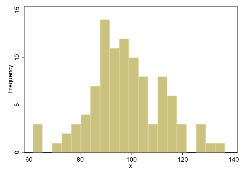
We can also run some histograms to confirm the normality of the distribution of these two variables. The histograms need to be run one at a time. Try:

hist x, bin(20) freq scheme(s1color)

And you get:

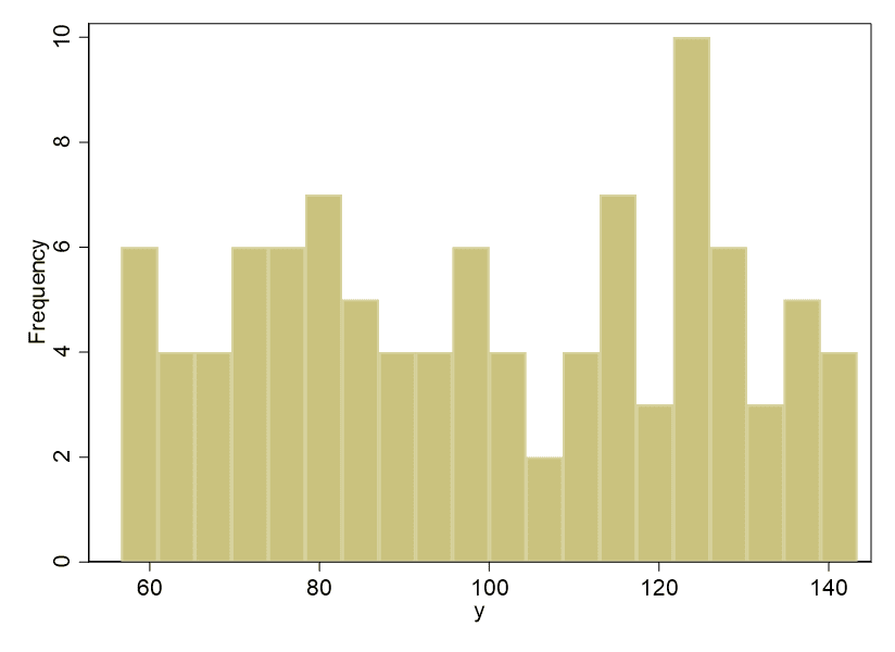
Next, try:

hist y, bin(20) freq scheme(s1color)

And you get:

The histograms confirm what the Shapiro-Wilk test told us, which is that x is distributed normally. Look at the classic bell curve shape of the histogram of x.

Variations

You can run the Shapiro-Wilk test on a subset of data. Let’s say you only wanted to run it for the first 50 values of x. Try:

swilk x in 1/50

And you get:

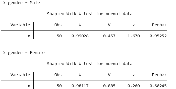
Let’s say you had a categorical variable, gender, for which you had x values, and you wanted to test the normality of x by category. Let’s create that category first, then run the Shapiro-Wilk test separately for the two values:

gen gender = 1
replace gender = 2 in 51/100
label define gender 1 "Male" 2 "Female"
label value gender gender
by gender, sort: swilk x

And you get: