Introduction
Analysis of variance (ANOVA) exists in order to determine whether there is an effect of an independent variable with more than two levels on a dependent variable that is continuously distributed. ANOVA can be accompanied by Tukey’s post hoc test in order to identify pairwise differences between individual levels of the independent variable. Don’t worry if that sounds complicated: This blog entry shows you how simple it is to carry out an ANOVA followed by Tukey’s test in R.
Load Dataset
Let’s load R’s built-in plant growth dataset:
data <- PlantGrowth
print(data)
These data measure plant growth as a function of three independent conditions or groups: (a) A control group, (b) treatment 1, and (c) treatment 2. The independent variable is group, the dependent variable is weight, and data is the name given to the data frame that holds these two variables.
Load Package
Let’s make sure you have gplots installed:
install.packages('gplots')
Run the ANOVA
Here’s the code for running the ANOVA in R on the selected data:
mod.aov <- aov(weight~group, data=data)
summary(mod.aov)
Results and Interpretation
Here are the results:

The ANOVA model is significant, F(2, 27) = 4.85, p = .0159.
However, on its own, this result only tells us that there is some effect of group on weight. We need the Tukey pairwise comparison in order to identify the magnitude and statistical significance of weight differences between the groups. Try the following code:
TukeyHSD(mod.aov)
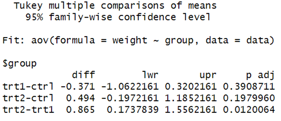
Here’s what you get:

Here we see that the only significant difference is between treatment 2 and treatment 1, p = .012. The mean weight associated with treatment 2 is 0.865 higher than the mean weight associated with treatment 1.
Graphing
Now let’s visualize the weight distributions as a function of group:
library("gplots")
plotmeans(weight ~ group, data = data, frame = FALSE,
xlab = "Treatment", ylab = "Weight",
main="Mean Plot with 95% CI")
 BridgeText can help you with all of your statistical analysis needs.


