Introduction
A one-sample t test is applied when you are measuring values of a single variable that you are comparing to some test mean. In this blog entry, we’ll show you how to conduct a one-sample t-test in Stata. You’ll also learn how to test for normalcy of distribution and create a 95% confidence interval graph for your data.
Create Data
First, we’ll create mock data, then we’ll show you how to test their normality, conduct a one-sample t-test, and generate a 95% CI plot. Let’s assume we’re measuring IQ for 1,000 subjects.
set obs 1000
gen subj = _n
label variable subj "Subject"
drawnorm iq_a, mean(100) sd(10)
gen iq = round(iq_a)
drop iq_a
label variable iq "IQ"
list in 1/30

Test for Normality
We’ll use the Shapiro-Wilk test to assess normality of IQ distribution in the sample, then create a histogram:
swilk iq
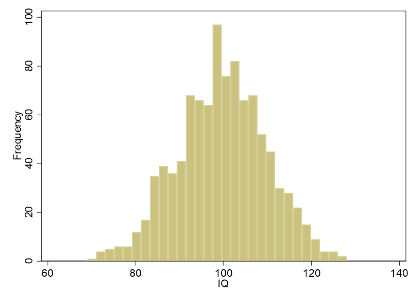
hist iq, freq scheme(s1color)

The null hypothesis for the Shapiro-Wilk test is normal distribution. The null hypothesis cannot be rejected, W = .99856, p = .59, so we assume normal distribution (if the distribution deviates significantly from normal, we can attempt the one-sample Wilcoxon signed rank test, which you can read about in a separate blog entry). The histogram demonstrates the normality of the distribution as well:

We can use sktest to separately assess for normality of skewness, kurtosis, and skewness and kurtosis:
sktest iq

In the skewness and kurtosis tests for normality, the null hypothesis is normality; examining the p values above, we cannot reject the null hypotheses for normality of skewness, kurtosis, and skewness and kurtosis.
The One-Sample t-Test
Now let’s run the one-sample t-test. We want to check if the sample mean differs significantly from 105, so we type:
ttest iq = 105
Here’s what we get:

Notice that we phrased the one-sample t-test as being two-tailed. In other words, we are checking for a difference from the test mean, not whether the sample mean is either greater than or less than the test mean. However, Stata helpfully gives us the one-tailed p values as well. In this case, there’s no practical effect, because the p for 105 being different from 99.56 (< .0001) is the same as the p for 105 being greater than 99.56 (p < .0001). However, in other contexts, p is likely to be different depending in the number of the tails in your hypothesis test, so that’s something to keep an eye on.
We reject the null hypothesis that 105 is not significantly different from the sample mean of 99.56, and, if we want to phrase this finding in a one-tailed manner, we could conclude that there is evidence that the sample mean of 99.56 (SD = 9.92) is significantly less than the test value of 105, t(999) = -17.36, p < .0001.
Graphic Support
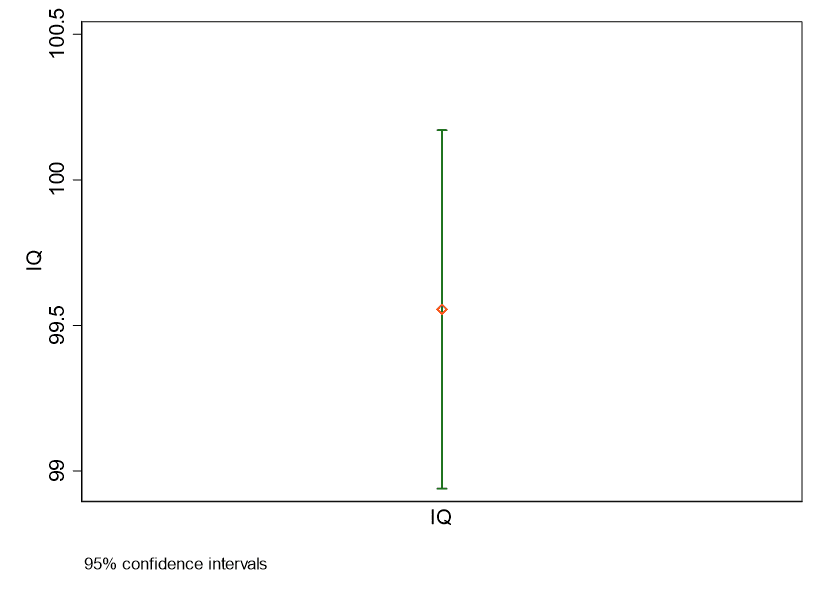
Finally, let’s illustrate the sample mean and 95% CI:
ciplot iq, scheme(s1color)
 BridgeText can help you with all of your statistical analysis needs.


