One-Sample t Test in R

Jan 14

Introduction

A one-sample t test is applied when you are measuring values of a single variable that you are comparing to some test mean. In this blog entry, we’ll show you how to conduct a one-sample t test in R. You’ll also learn how to test for normalcy of distribution and create a boxplot and histogram for your data.

Install Packages and Load Libraries

Install ggplot if you have not already done so, and load ggplot2:
install.packages("ggplot")
library(ggplot2)

Create Data

First, we’ll create mock data, then we’ll show you how to test their normality, conduct a one-sample t test, and generate a boxplot and histogram. Let’s assume we’re measuring IQ for 1,000 subjects.

iq2 <- rnorm(1000, mean=100, sd=15)
iq <- round(iq2)
sub <- 1:1000
iq_data <- data.frame(sub, iq)
head(iq_data)

Test for Normality and Create Histogram

We’ll use the Shapiro-Wilk test to assess normality of IQ distribution in the sample, then create a histogram:

shapiro.test(iq_data$iq)

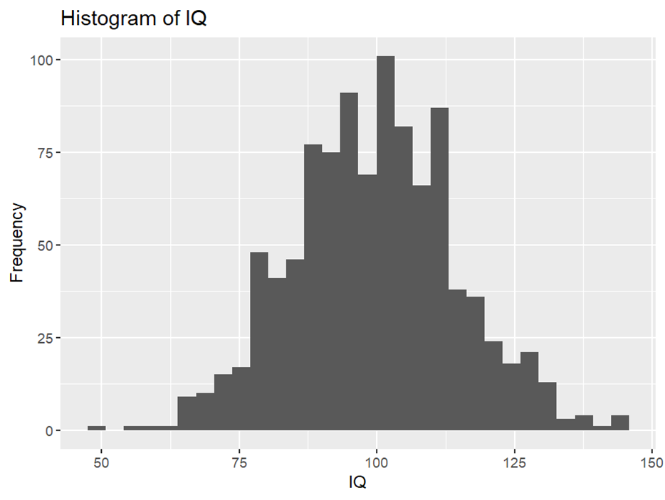
The null hypothesis for the Shapiro-Wilk test is normal distribution. The null hypothesis cannot be rejected, W = .99822, p = .39, so we assume normal distribution (if the distribution deviates significantly from normal, we can attempt the one-sample Wilcoxon signed rank test, which you can read about in a separate blog entry). The histogram demonstrates the normality of the distribution as well:

p <- ggplot(iq_data, aes(x=iq)) + geom_histogram()
p + labs(title="Histogram of IQ", y="Frequency", x="IQ")

The One-Sample t Test

Now let’s run the one-sample t test. Let’s begin by assuming a two-tailed approach in which:

H0: The mean IQ in the sample is not significantly different from 105.
HA: The mean IQ in the sample is significantly different from 105.

We want to check if the sample mean differs significantly from 105, so we type:

res <- t.test(iq_data$iq, mu = 105)
res

Here’s what we get:

Therefore, the sample mean of 99.531 is significantly different from 105, t(999) = -11.65, p < .0001.

We were checking for a difference from the test mean, not whether the sample mean is either greater than or less than the test mean. However, we could also have taken the following approach:

H0: The mean IQ in the sample is equal to or more than 105.
HA: The mean IQ in the sample is less than 105.

res2 <- t.test(iq_data$iq, mu = 105, alternate = "greater")
res2

Boxplot

Finally, let’s create a boxplot.

ggplot(iq_data, aes(y=iq)) + geom_boxplot(color="firebrick")