Introduction
The Cox proportional hazards model can be understood simply in terms of calculating the risk of an adverse event (hazard) as a function of some set of predictors. For example, death might be the hazard, and the use of a drug and the sex of a patient could be predictors. Quite often, in survival analysis, the goal is to understand the contribution of such predictors to the likelihood of the hazard. In particular, we might be interested in the effectiveness of treatments in reducing hazards.
In the Cox model, the hazard ratio has a protective function if under 1 and an exacerbating function if over 1. Let’s see the model in action in R.
Install Packages and Libraries
Install the following packages, if you have not done so already, and load them:
install.packages(c("survival", "survminer"))
library("survival")
library("survminer")
Load Data
Try the following code to load your data and examine its structure:
data("lung")
head(lung)
These are the results from a lung cancer survival dataset.

Run and Interpret the Model
In the model as structured, the hazard / failure event is dying. A code of 2 for status means that the person has died; a code of 1 means that the data are censored, meaning that the person was still alive at the time that data tracking ceased. To run the Cox proportional hazards model in R with sex as the independent variable of interest, enter the following code:
res.cox <- coxph(Surv(time, status) ~ sex, data = lung)
res.cox
summary(res.cox)

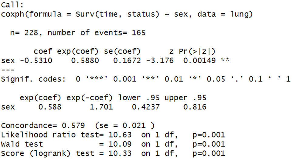
Here, we want to inspect the exponentiated coefficient for sex, which is 0.588. Because women are coded as 2 and men as 1, a woman’s hazard of dying is about 59% of that of a man. Note that this hazard ratio is statistically significant, p = .00149.
If this hazard ratio doesn’t make sense, consider a coding scenario in which men = 0, women = 1. In this case, take whichever variable is coded as 1, multiply it by the hazard ratio, and the resulting figure is a proportional hazard. In other words, a woman is (1)(0.588) = 58.8% as likely as a man to die.
You can add covariates to the Cox model. For example, if you wanted to add weight loss, you could try:
res2.cox <- coxph(Surv(time, status) ~ age + sex + wt.loss, data = lung)
summary(res2.cox)

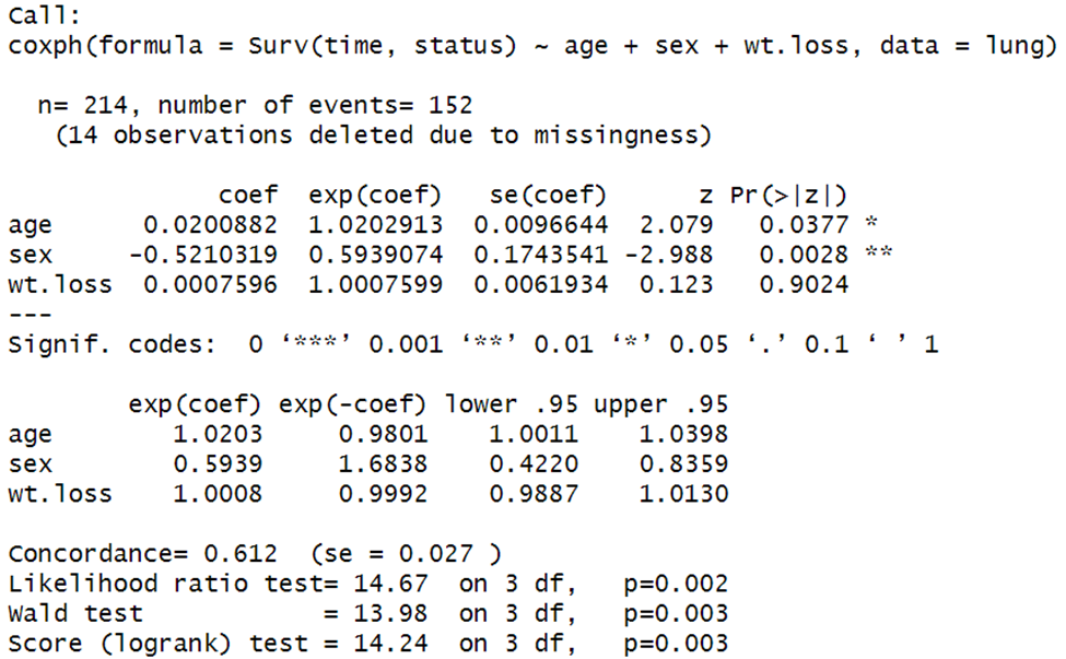
Every covariate you add will have an exponentiated coefficient and p value. Here, for example, we see that weight loss is not significant, p = .9024.
Graphical Support
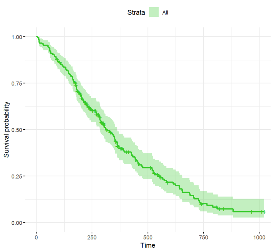
A natural next step in the analysis is to graph survival time, which we can do with the following R code:
ggsurvplot(survfit(res.cox), data = lung, color = "#36CA2A",
ggtheme = theme_minimal())

BridgeText can help you with all of your statistical analysis needs.


